
By Susan M. McMillan, PhD
Our 2003 paper on point-biserial correlations and p-values, item statistics from classical test theory, has been one of our most popular publications. This three-part blog provides a slightly revised and refreshed explanation for how item statistics can be used by educators to improve classroom assessments. Part 1 is a nontechnical overview of item analysis and explains why we recommend it for classroom assessments. Part 2 describes how to compute p-values and point-biserial correlations using an Excel spreadsheet, and Part 3 discusses the interpretation of item statistics.
Part 2: Computing P-Values and Point-Biserial Correlations
Some item banks and many learning management systems provide p-values and point-biserial (or item-total) correlations, so you may skip to “Part 3: Interpreting Item Statistics” of this blog series if you already have item statistics and aren’t interested in how they are computed. In this section, we present examples based on a fictional classroom test that is summarized in Figure 1.
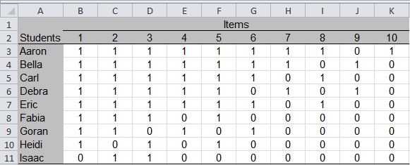
The student names are listed in rows 3 through 11 of column A, and the items are listed as the column headers (columns B through K) in row 2. All items are scored 0 if incorrect and 1 if correct. Each table cell contains the score that a student received on an item. For example, Aaron is the only student who got Item 10 correct (score of 1 in cell K3).
Computing P-Values
The p-value is the proportion of students who got an item with only two score points (correct or incorrect) correct. To compute the p-value, we need to sum the number of students who got the item correct and divide by the number of students who took the item.
Row 12 of Figure 2 demonstrates how to compute the p-value1. The cell with a heavy black border, B12, contains the formula shown in the formula bar at the top of Figure 2. When typing into cell B12, the equals sign tells Excel to expect a formula. The formula tells Excel to count the number of correct responses (count the number of “1s” in cells B3 through B11) and divide that total by the number of students with scores (count the number of numeric values in the same range of cells).
Copy the formula into cells C12 through K12 to get a p-value for each item.
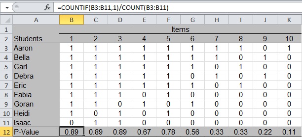
We can see that five students got Item 6 correct, and 9 students have numeric scores for the item, so 5/9 = 0.56, the value shown in cell G12. Notice that Item 10 is the most difficult (only one student got it correct), with a p-value of .11. Items 1, 2, and 3 were the easiest (eight out of nine students got them correct) with identical p-values of 0.89. Understanding how to use p-values is the topic of Part 3: Interpreting Item Statistics.
Computing Point-Biserial Correlations
The point-biserial correlation demonstrated here is the “corrected” item-total correlation; it excludes the item in question from the score total to avoid correlating the item score with itself.2 Making the correction adds a step to our process but avoids inflating the correlation.
In each figure, the formula bar at the top contains the formula typed into the cell that is highlighted with a heavy black border. The point-biserial calculation is made with the following steps:
- Compute the total score for each student by summing the item scores in columns B through K as shown in cell L3 of Figure 3. Copy the formula into cells L4 through L11.
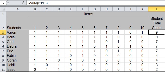
Figure 3: Compute the Total Score for Each Student - Compute the adjusted total scores by subtracting each item score from the total score as shown in cell M3 of Figure 4. (The item scores are not shown in Figure 4 for brevity; see Figure 3.) Copy the formula into cells M4 through M11 and then across the grid to fill each cell. The formula begins with “$L” to tell Excel to subtract from the value in the Total Score column as you copy the formula across columns.
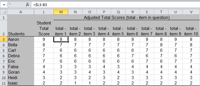
Figure 4: Compute the Adjusted Total Scores - Compute the corrected point-biserial correlation using the “correl” function in Excel as shown in cell M13 of Figure 5 (the p-values in row 12 are hidden in this figure). For Item 1 (the item scores are in columns B through K in Figure 3), the formula is telling Excel to correlate the
Item 1 scores in column B with the adjusted total scores in column M, which yields a point-biserial correlation of 0.46. Copy the formula across cells N13 through V13 to fill in the values for each item.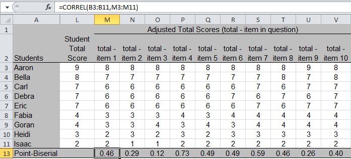
Figure 5: Compute the Corrected Point-Biserial Correlation
In our example test data, Item 4 has the highest point-biserial correlation (0.73 in cell P13), and Item 3 has the lowest (0.12 in cell O13). Understanding how to interpret point-biserial correlations is addressed in “Part 3: Interpreting Item Statistics.”
Footnotes
1. Computing an adjusted item mean (mean item score/maximum score possible) provides an estimate of item difficulty for constructed-response items, and the range is 0.0 to 1.0, like the p-value range.
2. Whether to use the corrected point-biserial correlation is not settled among assessment experts. The uncorrected item-total correlation will generally be higher but can still be a useful indicator of item discrimination.